Sponsored by Intel

Optimizing XGBoost Training Performance

XGBoost Just Keeps Getting Faster

by Egor Smirnov, Software Engineering Manager, and Kirill Shvets, Machine Learning Engineer, Intel Corporation

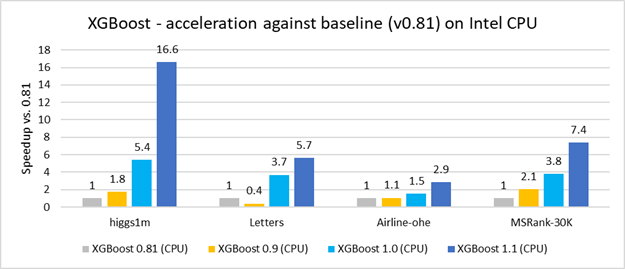
Optimizing XGBoost training is complex because many computational kernels require specific optimization techniques for irregular memory access, loops with dependencies, and branch mispredictions. That is why starting from XGBoost version 0.9 Intel began optimizing the XGBoost training stage. These efforts are paying off (Figure 1).

In this article we are going to compare performance of XGBoost 1.1 on CPU and GPU and have a closer look at the optimizations that were introduced for this release. Let’s start with a simple example of XGBoost usage.

A Practical Example of XGBoost in Action

The well-known handwritten letters data set illustrates XGBoost usage. This data set has 20,000 rows and 16 columns. Each row is described by 16 primitive numerical attributes (statistical moments and edge counts) that were scaled to fit a range of integer values from 0 through 15. Each row is associated with one of the 26 capital letters in the Latin alphabet. The XGBoost model is trained on 80% of the rows in the data set. The remaining 20% are used to test the model’s accuracy.

import gboost as xgb
import numpy as np# Set XGBoost parameters
xgb_params = {
   'alpha':            0.9,
   'max_bin':          256,
   'scale_pos_weight': 2,
   'learning_rate':    0.1,
   'subsample':        1,
   'reg_lambda':       1,
   'min_child_weight': 0,
   'max_depth':        8,
   'max_leaves':       2**8,
   'tree_method:       hist
}# Create DMatrix from the training set (in CSV format)
dtrain = xgb.DMatrix('letters_train.csv')# Train the model
model_xgb = xgb.train(xgb_params, dtrain, 1000)# Create DMatrix from the test set
dtest = xgb.DMatrix('letters_test.csv')
result_predict_xgb_test = model_xgb.predict(dtest)# Check model accuracy
acc = np.mean(y_test == result_predict_xgb_test)

Performance Comparison

Training performance is critical for models that have to be retrained often (e.g., as new data becomes available). As such, training time is compared for five real-world datasets:

• Higgs (1,000,000 rows, 2 classes)
• Airline-OHE (1,000,000 rows, 2 classes)
• MSRank (3,000,000 rows, 5 classes)
• Letters (20,000 rows, 26 classes)
• Abalone (4,177 rows, 28 classes)
• Abalone (4,177 rows, 28 classes)

We use the following AWS EC2 instances, each costs $3.06 per hour as of May 2020:

• Xeon: c5.18xlarge (Intel Xeon Platinum 8124M, 2 sockets, 18 cores per socket)
• V100: p3.2xlarge (NVIDIA Tesla V100)

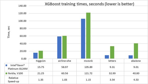
Figure 2 shows that training is up to 4.5x faster on the Xeon instance compared to an equivalently priced V100 instance. A cost comparison is shown in Figure 3. What we observe is that XGBoost training is not only faster on the Xeon instances compared to the V100 instance, it is on average 2x cheaper.

Intel Optimizations in XGBoost

The histogram tree-building method, which reduces the training time without compromising accuracy, is commonly used to solve large problems with a gradient-boosting model. Therefore, the histogram method for XGBoost training on is a prime optimization target.

Implementing this method is complex for the following reasons:

• It contains many kernels that impact execution time.
• It does not use BLAS, LAPACK, or any other common linear algebra functions that are already highly-optimized.
• Many kernels contain irregular memory access patterns, loops with dependencies, branch mispredictions, etc.

Consequently, XGBoost optimization prior to version 1.0 was limited. Since then, Intel has introduced many optimizations to maximize training performance. Three hotspots were identified for tuning: building histograms, partitioning, and evaluation of split (finding the best split). These optimizations and their effects on XGBoost training performance are discussed below. Note that the original source of all optimizations is the Intel Data Analytics Acceleration Library.

Building Histograms

Computation of gradients and Hessian matrices for training samples at each boosting iteration is performed by histogram building. The gradients and Hessian values can be summed into histogram bins according to the new discrete features. The task of finding the optimal splits for a decision tree is reduced to a simple problem of searching over the histogram bins in a discrete space.

XGBoost versions 0.81 and lower had a simple way to build histograms:

for (int i = 0; i < n; ++i) {
  for (int j = 0; j < p; ++j) {
    int bin = bins[row_idx[i] * p + j];
    hist[bin].g += g[i];
    hist[bin].h += h[i];
  }
}

To improve performance, we should consider parallelization, batch operations, and reducing memory consumption.

The histogram computation is easily parallelized by row blocks with a simple map pattern. As a result, there are partial histograms on each thread that are merged into a single histogram before finding the best split. In the previous implementation, splitting by the number of rows was too granular, meaning that sometimes too many small tasks were created when building the lower nodes of a decision tree. This created too much threading overhead. To reduce it, we increased the minimum task size for each thread.

In the ‘depthwise’ building mode, tree nodes of the same level are built in parallel. Batch functions are introduced to enable parallelism by nodes on the current level of a tree. This allows nested parallelism and improves scaling.

Histogram building is a memory-bound task, so reducing memory consumption can improve performance. To achieve this, we used data types that consume less memory. Input parameters were dispatched to one of the integer types (uint8_t, uint16_t, or uint32_t) based on the user-provided max_bin value. As a result, memory usage was reduced up to 1.5x with no accuracy loss.

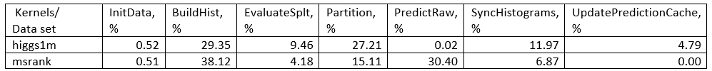
Before optimization, building histograms accounted for up to 82% of the training time. Now it consumes less than 50%. Table 1 shows the percent of the execution time attributed to each computational kernel in the XGBoost 1.1 release.

As you can see, after BuildHist, the Partition function is another hotspot. Let’s see what could be done to optimize it.

Partitioning and Finding the Best Split

Partitioning works like this:

1. After finding the best split (we have an index of the feature to split), run SplitIndex to split the sample in the current node into two descendents. This is known as SplitCondition.
2. Get the SplitIndex column.
3. Split the elements in this column into two subsets based on whether the element is less than SplitCondition. The first subset includes the indices of the elements that are less than SplitCondition, and the second contains the remaining indices.

The main problem with this kernel is finding opportunities for efficient parallelization. Here is the scheme that we used:

1. Divide the row index array among the threads.
2. Make a local partition in a local buffer.
3. Synchronize the threads to share the number of elements in each local partition.
4. Update the row index by copying the elements from the local buffers.

Conclusions

As a result of the XGBoost optimizations contributed by Intel, training time is improved up to 16x compared to earlier versions (Figure 1). Currently, XGBoost training on Xeon outperforms V100 at lower computational cost (Figures 2 and 3).

Software and Hardware Configurations

Algorithm Parameters

xgb_params = {
  'alpha':            0.9,
  'max_bin':          256,
  'scale_pos_weight': 2,
  'learning_rate':    0.1,
  'subsample':        1,
  'reg_lambda':       1,
  'min_child_weight': 0,
  'max_depth':        8,
  'max_leaves':       2**8,
  'tree_method:       hist,
  'n_estimators:      1000
}

Hardware Configuration

c5.metal AWS EC2 instance: Intel Xeon 8275CL processor, two sockets with 24 cores per socket, 192 GB RAM. OS: Ubuntu 18.04.2 LTS.

с5.18xlarge AWS EC2 instance: Intel Xeon Platinum 8124M processor, two sockets with 18 cores per socket, 144 GB RAM. OS: Ubuntu 20.04 LTS.

p3.2xlarge AWS EC2 instance: CPU: Intel Xeon E5–2686 v4 processor; GPU: Tesla V100-SXM2–16G (driver version: 410.104, CUDA version: 10.0), 61 GB RAM. OS: Ubuntu 18.04.2 LTS

Testing date: 05/18/2020

Software Configuration

XGBoost — release 1.1 build from sources.

Other software: Python 3.6, NumPy 1.16.4, pandas 0.25, Scikit-learn 0.21.2.